It seems that many publications nowdays focus on Solving application problems eg. Vision, Motion, Code with the assumption that the backbone of these models are already optimized.
But to my opinion, there are still a lot of room for imporvement and optimization, which would probably solve the shortage of Hardware (GPUs) with much faster and efficient learning and inference.
“Intelligence manifests most clearly when you can do a lot with little in terms of input.” - David Krakauer
Backbone ideas are from the video of Welch Labs Why Deep Learning Works Unreasonably Well
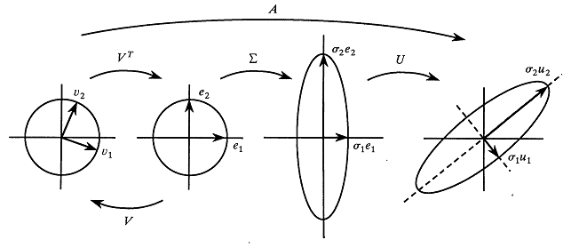
A Neural Network can be bluntly seen as a Matrix-Multiplication process. Which transforms a input-vector to a output-vector. But how does this transformation make sense? What does it mean by transformation?
The above SVD(Singular Vector Decomposition) figure shows what it does. ($U$) and ($V^T$) Rotates the input-vector as they are Orthogonal Matrices, and ($Σ$) Scales each element in the vector as it’s a Diagonal Matrix.
So, the transformation can be interpreted as a Selective information transformation.
But this only scratches the surface of what a Neural Net actually does. There must also be the clarification of what a Hidden Layer does, and the Activation function does.
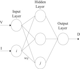
Hidden Layer
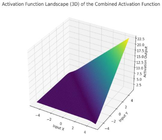
Activation Layer Visualization
MLPs, so well used nowdays are overlooked in its mechanism, which was actually a crucial breakthrough that solved the famous XOR problem. A hidden layer is a simple concept of sequentially applying N number of matrix multiplication. But as we all know, \(W₂(W₁x + b₁) + b₂ = (W₂W₁)x + (W₂b₁ + b₂)\) shows that any sequential number of matrix multiplication can always be represented as a single layer of matrix multiplication. So how does a hidden layer exist? Activation functions.
Before Neural Networks, SVMs were a great way to solve classification problems. Apart from the soft vectors margin algorithm that created robust classifiers, there was another method that made huge breakthroughs. Kernel maps, which projected input data into high dimensional space solved many non-linear problems. From Polynomial Kernels to Gaussian Kernels, each non-linear map was used to extract non-linear complex features to classify it’s data.
Activation functions are these kind of non-linear maps that enable Matrix Systems to learn much more complex structure or features. The above figure shows the geometrical folding of feature spaces that these activation functions apply.
There are a lot of discussions and improvements needed on this activation function. which i believe is a crucial part in optimization such as Sparsity, Ordinary Differential Equations, Kernels.. Will Come back to it in another post.
So a Neural Network is a system that uses non-linear function to learn complex features from input data with Selective information transformation and geometrical folding. But there are so many other things known and unknown that enables Neural Networks to perform extreemly well.
The most important feature must be Depth.

Backbone ideas are from the Article in Lesswrong A Simple Introduction to Neural Networks
A simple but not 100% technical answer is that, models learns by reversing the hierachical generation process of nature. Think of a generation of face process for example. We create a face first with the shape, the location of eyes, nose and lips .. and than decide on the detail of these organs. The famous AlexNet that opened the possibility of Deep Neural Networks also shows Hierachical Detectors where curve detectros in the earlier layers create ear detectors in the later layers. So each layers devides the features needed to learn by models into more specific and divers features.(You can also think of Dynamic Programming, which divides the problem into sub-problems)
For Specific explanations, i would recommend reading this article from Chris Olah Zoom In: An Introduction to Circuits.
Another way of putting it is by using the terminology of complexity and regions. We can view a Matrix as a transformation of coordinates of input vectors in parameter space. For example, a A : [[0,1] , [1,0]] Matrix swaps the x and y axis of the input vector [x, y] into [y,x]. In this view, we can think of these activation functions and matrices as shifting of coordinates of input vectors into different regions to classify what region each point resides in.
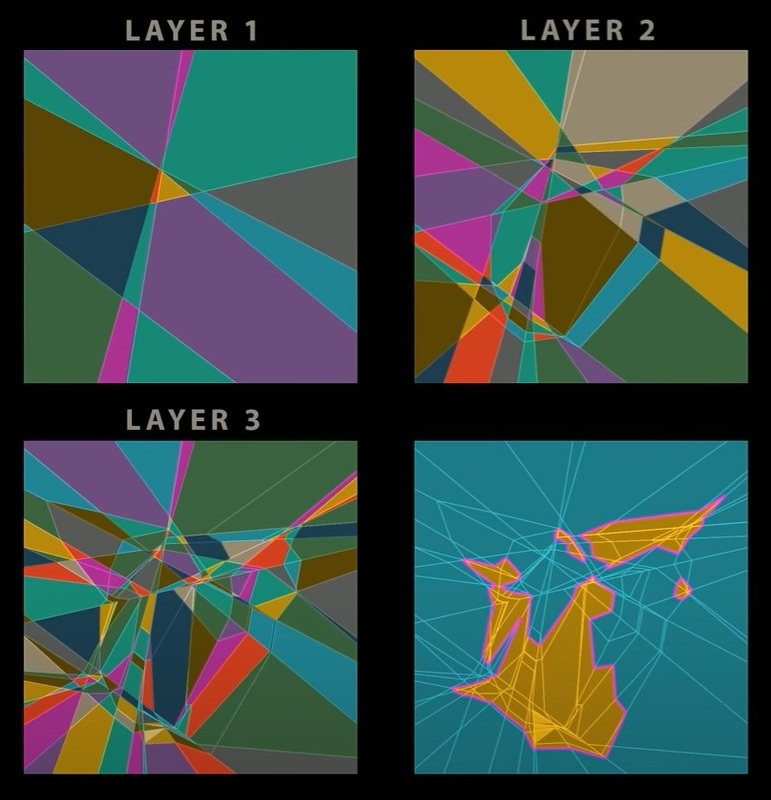
A Screen shot from the video of Welch Labs
Think of a highly expressive n category classifier such as SVMs or Decision Trees. These models devide the output space into n regions, which are (if trained well) 1:1 to each categories (Region for A/B/C/D…). In a Neural Network, this region is made in each layers for categories, features and many other complex measures, and this number grows exponentially with depth.
\[N_r = \prod_{k=1}^{K-1} \left( \frac{D}{D_i} + 1 \right)^{D_i} \sum_{j=0}^{D_i} \binom{D}{j}\]The above formula is from Understanding Deep Learning-Prince(2023).
\(N_r\) is the number of regions for \(K\) layers, where \(D\) is the number of hidden units in each \(K\) layers and \(D_i\) is the input dimension of the vector. So for classifying various outputs, the variety of representation exponentially grows with depth (\(K\)). But there are still many things to know like Initialization, Interpolation, Stability. Like, if things were this simple, Deep learning may have worked since the 2000s.
I’m not going to talk about the characteristics and differences between width and depth for now. Just know that width increases (though quite obvious) the dimension of the hidden states, meaning that the hidden units have more degree of freedom. A NN which needs compression decreases dimension, and increases dimension if more and complex information expansion is needed from the input vector. (Some papers say depth is more important than width, i agree if there is a optimizer)
So now we have the matrices and activation functions, and we also know that big neural networks perform well. Most people say that it was the GPUs that made NN possible, but this is only half true. To know why this architecture was possible, we should definetly demystify it’s learning algorithm, Gradient Descent and Backpropagation.
From the lecture of IDEAS AND COMPUTATIONS IN THE FIRST ORDER OPTIMIZATION by professor Woocheol Choi at SKKU.
Many think of Gradient Descent as a algorithm from Machine Learning, but this is devastatingly wrong. This method is a very old calculus method which was invented to find the minimum of a certain function, also known as the convex optimization problem.
Before talking about Backpropagation and chain rules, there must be at least some understanding of the basic formula of Gradient Descent, which later shows why we need Batch Normalization, and how Momentum based optimizers(ADAM) actually work.
The formula below is from the lecture note on convex optimization by professor Woocheol Choi from SKKU.
\[\min_{x \in \mathbb{R}^n} f(x)\] \[x_{t+1} = x_t - \eta \nabla f(x_t)\]So this is the formula we all know, the ball $x_t$ goes down the sloap with the information from gradient $\eta \nabla f(x_t)$. But why does this formula work? As i don’t have a degree in Mathematics, my answer might not be sufficient. So i bring the explanation from my college professor, who proved by using Taylor expansion.
\[f(y) - f(x) = \int_x^y f'(s)ds \quad (1.9)\] \[f(y) \leq f(x) + (y - x)f'(x) + \frac{|f''(x)|}{2}(y - x)^2 \quad (1.15)\]This is where the $\text{second order taylor expansion}$ is used. The proof between (1.9) ~ (1.15) was skipped. Just for now. (Actually, the original proof takes extra steps with another huge assumption that \(|f''(x)| \leq C\) which later refers to (1.16) using $O$, a constant insted of $|f’‘(x)|$. )
$\text{This is where Normalization is needed! }$ To ensure that \(|f''(x)| \leq C\) holds for the function $f$ to find the minimum with the \(|f''(x)|\) function staying in the upper-bound of constant $C$. And is so called as $ \beta \text{ smoothness.} $ (I think there are other explanations too in this Batch Normalization theory, but for now i will focus on the effect in terms of gradient descent)
\[f(y) = f(x) + (y - x)f'(x) + O\left((y - x)^2\right) \quad (1.16)\] \[\text{and if } y \approx x\text{, then}\] \[f(y) \approx f(x) + (y - x)f'(x) \quad (1.17)\] \[\text{Inserting } y = x_{t+1} \text{ and } x = x_{t} \text{ with } x_{t+1} = x_t - \eta \nabla f(x_t) \text{, we find }\] \[f(x_{t+1}) \approx f(x_t) - \eta |f'(x_t)|^2 \quad (1.18)\]So now we can see that $f(x_{t+1})$ decreases from $f(x_t)$ as the gradient descent takes place as \(x_{t+1} = x_t - \eta \nabla f(x_t)\) .
There are so many other things to talk about such as loss landscape, global & local minima, sharp & flat minima, eigenvalue-distribution and baysin priors. But they will be discussed in a later post.
But we are not searching for a minima of simple $f$. We are searching for a minima of \(f = \sigma_\ell \circ h_\ell \circ \cdots \circ \sigma_2 \circ h_2\) where $h$ is a hidden layer function and $f$ is a composite function. So we expand the Gradient Descent with Back propagation consisting of chain rules.
Backbone ideas are from the post by Andrej Karpathy Yes you should understand backprop and again Welch Labs The F=ma of Artificial Intelligence [Backpropagation, How Models Learn Part 2].
A multiple layer of matrices with activation functions(non-linear maps) using gradient descent to find the solution that minimizes the function (more specifically cost or loss functions. MSE, Cross-Entropy, ELBO… Will come back in another post) output needs to be optimized. Think of a Netowrk with 2 layer of [4608, 9216] x σ x [9216, 10] matrices with a cross-entropy loss function.
The input is a [2,48,48] image and you want to classify what digit label the image has. If there was no back-propagation to use, i would have think of a heuristic way of solving this problem. (eg. devide the image by pixel groups, encode weights to detect shapes, sum up the scores, check the errors and search for a better algorithm).
The early neural nets were trained in this way, by twiking the values of weights by real human experts. But this is impossible if we have $10$ to $20$ layers ([4608, 9216] x σ1 x [9216, 9216] x σ2 x [9216, 9216] x … x σ20 x [4608, 10]), which means it is not scalable.
Then can we describe each element of the matrix components as a mathematical formula and find the solution to that formula? This is where the chain rule comes in.
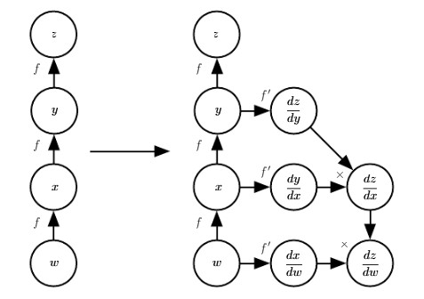
deeplearningbook chapter 6.
But before showing the chain-rule, the gradient descent formula must be more clarified since it’s not just $f$ we are optimizing.